Examples
The code below simulates an area of 1 hectare. Starting from a treeless landscape, every year seeds on the seed bank have the change to germinate. The simulation goes on for 300 years
import trees_ibm
import matplotlib.pyplot as plt
import numpy as np
import random


#################################################################
#                          PFT CREATION                         #
#################################################################

par_1=dict(
    wood_density=0.35,
    max_agb=200,
    max_dbh=145,
    h0=3.3,
    h1=0.60,
    cl0=0.80,
    cd0=0.60,
    cd1=0.68,
    cd2=0.0,
    rho=0.55,
    sigma=0.70,
    f0=0.77,
    f1=-0.18,
    l0=2.0,
    l1=0.10,
    Iseed=0.03,
    Nseed=20,
    m=0.5,
    rg=0.25,
    Mb=0.015,
    pmax=2,
    alpha=0.36,
    Dmort=10,
    Dfall=0.45,
    pfall=0.3,
    DdeltaDmax=0.33,
    deltaDmax=0.012,
    m_max=0.12,
    Fdisp=1.0,
    Adisp=0.118,
    Nfruit=30)


par_2=dict(
    wood_density=0.35,
    max_agb=200,
    max_dbh=58,
    h0=4.6,
    h1=0.4,
    cl0=0.80,
    cd0=0.60,
    cd1=0.68,
    cd2=0.0,
    rho=0.55,
    sigma=0.70,
    f0=0.77,
    f1=-0.18,
    l0=2.0,
    l1=0.10,
    Iseed=0.01,
    Nseed=15,
    m=0.5,
    rg=0.25,
    Mb=0.03,
    pmax=3.1,
    alpha=0.28,
    Dmort=10,
    Dfall=0.45,
    pfall=0.3,
    DdeltaDmax=0.34,
    deltaDmax=0.012,
    m_max=0.12,
    Fdisp=1.0,
    Adisp=0.118,
    Nfruit=30)

par_3=dict(
    wood_density=0.35,
    max_agb=200,
    max_dbh=58,
    h0=4.8,
    h1=0.4,
    cl0=0.30,
    cd0=0.60,
    cd1=0.68,
    cd2=0.0,
    rho=0.41,
    sigma=0.70,
    f0=0.77,
    f1=-0.18,
    l0=2.0,
    l1=0.10,
    Iseed=0.05,
    Nseed=21,
    m=0.5,
    rg=0.25,
    Mb=0.03,
    pmax=6.8,
    alpha=0.23,
    Dmort=10,
    Dfall=0.45,
    pfall=0.3,
    DdeltaDmax=0.23,
    deltaDmax=0.019,
    m_max=0.12,
    Fdisp=1.0,
    Adisp=0.118,
    Nfruit=30)

par_4=dict(
    wood_density=0.35,
    max_agb=200,
    max_dbh=44,
    h0=4.3,
    h1=0.4,
    cl0=0.30,
    cd0=0.60,
    cd1=0.68,
    cd2=0.0,
    rho=0.40,
    sigma=0.70,
    f0=0.77,
    f1=-0.18,
    l0=2.0,
    l1=0.10,
    Iseed=0.02,
    Nseed=50,
    m=0.5,
    rg=0.25,
    Mb=0.04,
    pmax=11,
    alpha=0.20,
    Dmort=10,
    Dfall=0.45,
    pfall=0.3,
    DdeltaDmax=0.60,
    deltaDmax=0.029,
    m_max=0.12,
    Fdisp=1.0,
    Adisp=0.118,
    Nfruit=30)

par_5=dict(
    wood_density=0.35,
    max_agb=200,
    max_dbh=16,
    h0=4.3,
    h1=0.3,
    cl0=0.30,
    cd0=0.60,
    cd1=0.68,
    cd2=0.0,
    rho=0.52,
    sigma=0.70,
    f0=0.77,
    f1=-0.18,
    l0=2.0,
    l1=0.10,
    Iseed=0.03,
    Nseed=50,
    m=0.5,
    rg=0.25,
    Mb=0.021,
    pmax=7,
    alpha=0.30,
    Dmort=10,
    Dfall=0.45,
    pfall=0.3,
    DdeltaDmax=0.33,
    deltaDmax=0.011,
    m_max=0.12,
    Fdisp=1.0,
    Adisp=0.118,
    Nfruit=30)


par_6=dict(
    wood_density=0.35,
    max_agb=200,
    max_dbh=16,
    h0=3.0,
    h1=0.60,
    cl0=0.30,
    cd0=0.60,
    cd1=0.68,
    cd2=0.0,
    rho=0.47,
    sigma=0.70,
    f0=0.77,
    f1=-0.18,
    l0=2.0,
    l1=0.10,
    Iseed=0.02,
    Nseed=50,
    m=0.5,
    rg=0.25,
    Mb=0.045,
    pmax=12,
    alpha=0.20,
    Dmort=10,
    Dfall=0.45,
    pfall=0.3,
    DdeltaDmax=0.60,
    deltaDmax=0.029,
    m_max=0.12,
    Fdisp=1.0,
    Adisp=0.118,
    Nfruit=30)


FT1=trees_ibm.trees_ibm.Tree.TreeFactory(new_cls_name="FT1", new_parameters=par_1)
FT2=trees_ibm.trees_ibm.Tree.TreeFactory(new_cls_name="FT2", new_parameters=par_2)
FT3=trees_ibm.trees_ibm.Tree.TreeFactory(new_cls_name="FT3", new_parameters=par_3)
FT4=trees_ibm.trees_ibm.Tree.TreeFactory(new_cls_name="FT4", new_parameters=par_4)
FT5=trees_ibm.trees_ibm.Tree.TreeFactory(new_cls_name="FT5", new_parameters=par_5)
FT6=trees_ibm.trees_ibm.Tree.TreeFactory(new_cls_name="FT6", new_parameters=par_6)

##################################################################

database_name="example_1.h5"

topology=trees_ibm.Tree_Grid(x_max=5,y_max=5,delta_h=0.5,patch_area=400,I0=860,lday=12,phi_act=365,k=0.7)
world=trees_ibm.Tree_World(topology=topology)

world.create_HDF_database(database_name)

world.initial_update()
dispersal_settings={'mode':'external',
                    'clear':False}

world.run_simulation(n=3600,dispersal_settings=dispersal_settings,h5file=database_name)
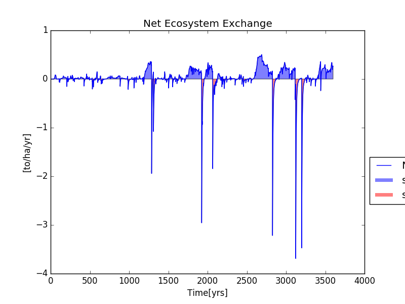
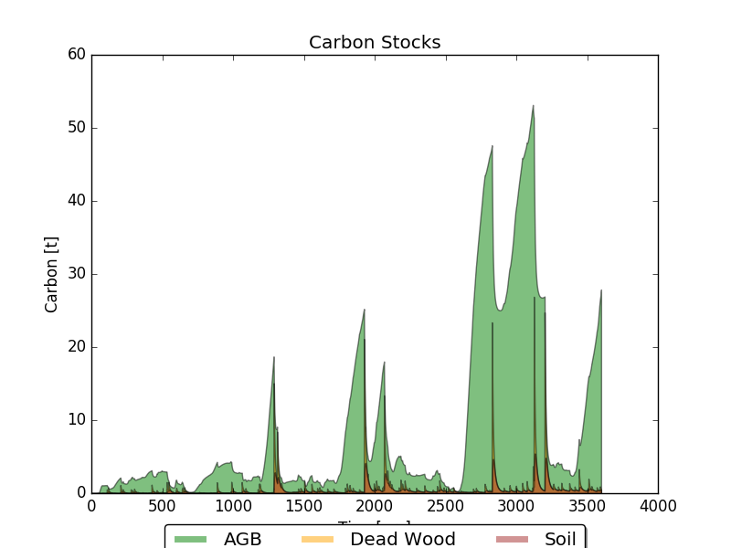
All the data generated during the simulation is now stored in the HDF5 database. We can access this data to run analyses or simply visualize some aspects of our simulation. The code below the Net Ecosystem Exchange and Carbon Stocks using one of the plotting functions available in the visualization module within trees_ibm.
from trees_ibm.visualization import plot_NEE, plot_stocks
import matplotlib.pyplot as plt
from tables import open_file
database_name="example_1.h5"


h5file=open_file(database_name,"r")
nee_table=h5file.root.sim_1.trees.sys_lvl.NEE
nee=nee_table.col("nee")
plot_NEE(nee)
fig_name="NEE_"+database_name.split(".")[0]+".png"
plt.savefig(fig_name,format="png")

Stocks={"AGB":[],"Dwood":[],"Sfast":[],"Sslow":[]}
stocks_table=h5file.root.sim_1.trees.sys_lvl.Stocks
Stocks["AGB"]=stocks_table.col("agb")
Stocks["Dwood"]=stocks_table.col("dead_wood")
Stocks["Sfast"]=stocks_table.col("soil_fast")
Stocks["Sslow"]=stocks_table.col("soil_slow")
plot_stocks(Stocks)
fig_name="Stocks_"+database_name.split(".")[0]+".png"
plt.savefig(fig_name,format="png")

h5file.close()